NGC2264

The Cone Nebula (and why I decided to spend my Christmas nights like this)

The Christmas tree nebula photographed in different wavelengths

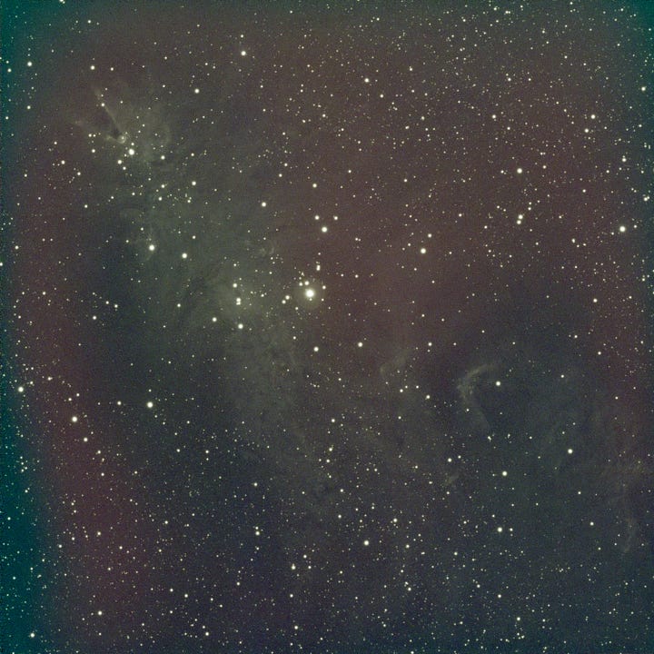
The Cone Nebula, catalogued as NGC 2264 in the New General Catalogue, is a large cloud of interstellar gas and dust in the constellation Monoceros. Its overall shape can resemble a Christmas tree—especially if you’re observing from the Southern Hemisphere, where it appears “upright”, with the apex at the top—hence the other name it’s often associated with: the Christmas Tree.
It also happened to be one of the four imaging projects I worked on during the Christmas period, which—this time—felt weirdly appropriate.

Since I got into deep-sky astrophotography four years ago, this was my first real chance to tackle a full narrowband project in a structured way: capturing (separately) the main emission lines typically used for this kind of target, and then combining them into different color palettes. It’s a very common technique in advanced amateur astrophotography, and I’ve only started exploring it seriously in the last months.
NGC 2264 is a great target for this, because it contains strong emissions from ionized hydrogen (Hɑ), doubly ionized oxygen (OIII), and ionized sulfur (SII), three of the classic channels used to build narrowband color images.

In general, capturing separate emission bands gives you the option to combine them in different “palettes” by mapping each band to the R, G, and B channels of the final image. For example: assign SII to red, Hα to green, and OIII to blue. Swap the mapping around and you’ll emphasize different structures and physical regions of the nebula—features that can otherwise be hidden or diluted.
This is also the general idea behind many of the iconic astronomical images we’re used to seeing from professional observatories (including space telescopes): there’s even a well-known rendering style called the Hubble palette, whose name has been taken from the Hubble telescope in orbit around the Earth.

With a monochrome camera, this is conceptually straightforward: each filter produces a grayscale image representing the intensity of that specific wavelength.

With a one-shot color (OSC) camera like my astronomical camera or common DSLRs, it gets a bit more nuanced. Even if you use narrowband filters, the sensor still records the light through a Bayer matrix (R/G/B microfilters), so the signal ends up distributed across the RGB channels according to the sensor’s color filter response. In practice, one channel usually dominates for a given emission line—but some amount of the signal can still leak into the other channels and anyway you get color images.

I won’t dive here into the eternal “are these colors real or fake?” debate (I get that question a lot). It’s not a great question as stated. We’re still dealing with visible light emissions—OIII really is in the blue-green/cyan part of the spectrum, Hα is deep red—but the key issue is how much of what we see (or map) in an image corresponds to isolated emission lines vs. broadband light, and how we choose to represent those components in a final RGB rendering. Maybe I’ll do a dedicated post about that. For now the honest answer is: it depends, and the “truthfulness” depends on the specific mapping and on what you mean by “true”.

This long preface is unnecessary if you do astrophotography, but it’s useful for anyone who loves the images and wants to understand what’s behind them. From here on, we go technical: proceed at your own risk—boredom guaranteed.

Acquisition setup and dataset

A few notes about the setup I used to get my images:

• Mount: SkyWatcher EQ6R-Pro (equatorial)

• Camera: ZWO ASI533MC Pro, cooled to −10°C

• Telescope: TS-Optics AP 115/800 ED Photoline

• Reducer/Flattener: Starizona Apex ED 0.65× L

• Guiding: TS-Optics Guidescope Deluxe 60 mm + ZWO ASI290MM Mini

• Controller: ZWO ASIAIR Plus

• Autofocus: ZWO EAF

• Filters (2”): Optolong L-PRO, Optolong L-eXtreme, SVBONY SV227 OIII 5 nm, SVBONY SV227 SII 5 nm

Over 12 non-consecutive nights between December 27, 2025 and January 12, 2026, I collected:

• Optolong L-PRO (broadband) filter: 139 × 60s photographs ≈ a bit over 2 hours - Used mainly for stars (full visible spectrum) and as a broadband reference/luminance component.

• Optolong L-eXtreme (dual band Hα + OIII, 7nm) filter: 356 × 300s photographs ≈ just under 30 hours - Captures mostly Hα and a portion of OIII.

• Svbony SV227 OIII (5 nm) filter: 41 × 600s photographs ≈ about 7 hours - Dedicated OIII acquisition.

• Svbony SV227 SII (5 nm) filter: 214 × 300s photographs ≈ about 18 hours - Dedicated SII acquisition.

Total exposure time across bands: about 57 hours.

For anyone who doesn’t do astrophotography and somehow made it this far: yes, this means I photographed that patch of sky for ~a dozen nights, collecting nearly 700 pictures, or “light frames”, at different exposures depending on the filter. I also captured 151 bias frames, 41 dark frames for each exposure length (60s, 300s, 600s), and 51 flat frames for each of the 12 acquisition sessions. That’s the raw base.

Context note for astrophotographers: I image under a Bortle ~7 sky. The reason I have fewer OIII hours than the other channels is simply that after the first OIII night (the last filter in my plan), the weather turned into a multi-day mess. At that point I decided to stop acquiring, move to processing, and close the project.

Processing was done mostly in PixInsight (calibration, registration, integration, band combination, stretching, finishing). I used Photoshop only for some final local color/contrast tweaks and for star reintegration—something you can do in PixInsight too, but I personally find it faster and more controllable in Photoshop.

For brevity, I’ll refer to the four datasets as:

• LPRO (broadband)

• LXT (L-eXtreme dual band)

• OIII (SV227 OIII narrowband)

• SII (SV227 SII narrowband)

Processing workflow in PixInsight

As a general approach, I usually process stars and background separately, especially for projects like this. After images integration and preliminary cleanup, I separate the stars from the nebula and continue working on the two images independently. I add the stars back only at the end (in Photoshop). This gives much better control across the whole workflow.

That being said, these are the steps in PixInsight.

1. Light calibration → cosmetic correction → debayer. Since I already had the required bias and dark libraries, I integrated only the flats from each session to generate the master flats, then calibrated and debayered each dataset separately.

2. SubframeSelector (SS) + outlier rejection
   For each set I ran SubframeSelector and assigned weights to images using Juan Conejero’s formula. I also inspected the statistical distributions of FWHM, eccentricity, PSF SNR, median, and altitude indexes through the datasets to reject obvious outliers:

   • For LPRO (used mostly for the star field), I rejected frames with FWHM/eccentricity clearly outside the main cluster—indicative of focus issues, guiding problems, satellite/meteor trails, etc. I kept only frames likely to produce sharp, round stars.

   • For LXT, I rejected frames with clearly poor combined median/altitude/PSF SNR, to avoid integrating “dirty” signal caused by haze, residual clouds, light pollution variations, dawn proximity, etc.

   After SS, I kept 121 LPRO frames and 301 LXT frames.

   I did not reject frames from OIII (already a small set) and SII (quite homogeneous). I let the weighting handle quality variation.

3. LocalNormalization (LN) on LXT, OIII, SII
   I applied LocalNormalization to equalize gradients and normalize frames inside each dataset, using an internal reference.

   • For OIII (single night, only 41 frames), I used the highest-weight frame as reference.

   • For LXT and SII, I integrated roughly the top ~18% best-weighted frames to build a reference image for LN.

   I used PixInsight’s default LN parameters; in particular I kept:

   • Scale = 1024 (to target large-scale gradients/haze)

   • Minimum detection SNR = 40.0 (since all frames had a clear star field even in narrowband).

   I did not apply LN to LPRO, because my main interest there was extracting stars, not producing a perfect broadband background integration.

4. StarAlignment

   I registered all frames to a common geometry so that all datasets (LXT, OIII, SII, LPRO) were perfectly co-registered before integration and later combination.

   • Reference frame: I used the highest-weight subframe from the LXT dataset as the single global reference.

   • Targets: I aligned each dataset to that same reference, keeping the registered outputs separated by filter/dataset to avoid mixing intermediate products across steps.

   • Settings: I used PixInsight’s default StarAlignment parameters.

   • Drizzle: After a few experiments I disabled drizzle. In theory, 2× drizzle was the only option that could make sense here; in practice it introduced strong checkerboard artifacts in the SII and OIII datasets (while LXT looked fine), so I dropped it to keep the results consistent across filters.

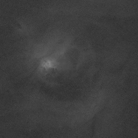
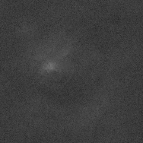
5. ImageIntegration → four color masters
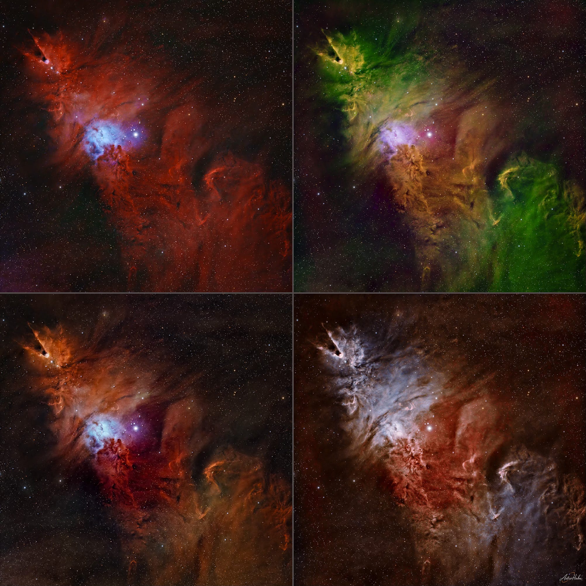
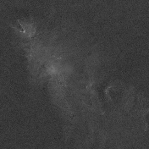
   I integrated each dataset separately, producing four color masters:

   • LPRO_master: broadband image (L-PRO filter is designed to suppress common urban light pollution bands and improve contrast under light-polluted skies). In this master, all RGB channels contribute meaningfully, and the result is broadly representative of what we’d see if the nebula were bright enough to register visually.

   • LXT_master: dual-band Hα + OIII combined. The dominant red comes from Hα; the OIII signal typically contributes mostly to the green/blue side.

   • OIII_master: OIII-only dataset. This tends to look cyan/blue-green. The red channel is essentially noise, while green/blue carry most of the usable OIII signal. In my case, this master is also limited by the fact that I only managed one night of OIII.

   • SII_master: SII-only dataset. SII is in deep red, so the red channel dominates; blue is usually negligible and largely noise.

     

     

     From left to right, from top to bottom: LPRO_master, LXT_master, OIII_master, SII_master

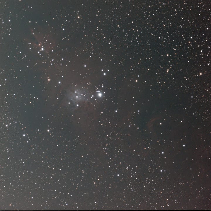
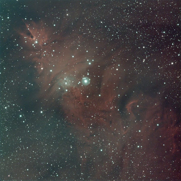
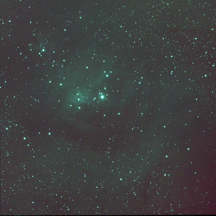
   All these images are shown with PixInsight ScreenTransferFunction (STF): an automatic screen stretch for visualization only, without modifying the actual pixel values. Without STF they would look almost black, with only a handful of bright stars.

6. Preprocessing of master images
   On LPRO_master and LXT_master I ran:

   • ImageSolver (astrometric solution)

   • SpectroPhotometricFluxCalibration (SPFC; requires ImageSolver)

   • DynamicBackgroundExtraction (DBE)

   • BackgroundNeutralization (BN)

   • SpectroPhotometricColorCalibration (SPCC)

     (color calibration based on astrometry + filter response + catalogs)

   • BlurXTerminator (BXT)

     (deconvolution/sharpening for stars and nebula microcontrast)

   • StarXTerminator (SXT)

     to split stars and background

   From there:

   • I discarded the stars extracted from LXT_master

   • I kept the stars extracted from LPRO_master as the most “natural” visible-light star field

   So I ended up with three color images:

   • LPRO_starless

   • LPRO_stars

   • LXT_starless

   Then, since OIII_master and SII_master are effectively monochrome data carried in an RGB container (and don’t require full photometric color calibration), I applied only:

   • DBE

   • BN

   • SXT (keeping only the starless images)

   Eventually resulting with two more color images:

   • OIII_starless

   • SII_starless

7. ChannelExtraction on the starless masters
   At this point, with the stars removed from each master, I used ChannelExtraction to split each RGB image into its three monochrome components.
   Even though these narrowband datasets are stored as RGB images (because the camera is one-shot color), it’s very useful to look at the channels separately: each extracted channel is effectively telling you how much signal the camera recorded through that filter as seen by the red/green/blue elements of the sensor.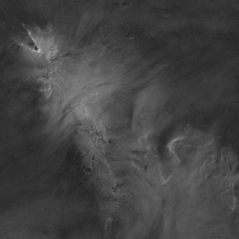

   

   

   

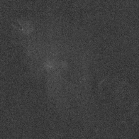
   From left to right, from top to bottom: LXT_R, LXT_G, LXT_B, OIII_R, OIII_G, OIII_B, SII_R. SII_G, SII_B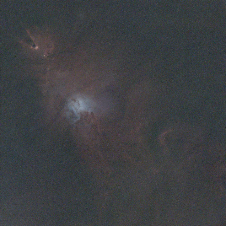

   

   LPRO_starless and LPRO_stars

   This is where the physics starts becoming visible even before any palette work.
   By looking at the individual channels extracted from the narrowband starless masters, you can already see quite clearly how differently the nebula behaves at each wavelength. In particular, ionized hydrogen (Hα) contributes essentially nothing in the blue channel, while doubly ionized oxygen (OIII) shows up almost entirely in the green and bluechannels.
   This is exactly why the L-eXtreme dataset (LXT)—which captures Hα and part of OIII—produced a master with a very strong red channel and only a moderate contribution in green and blue.
   Likewise, the SVBONY SV227 OIII dataset produced an image whose red channel is effectively empty, which is fully consistent with the spectral characteristics of OIII emission. Finally, the SVBONY SV227 SII dataset—targeting ionized sulfur, which lies in the deep red—produced a master where the red channel is strongly dominant and bright, while the other channels carry mostly weak residual signal and background noise.
   Because of this, and to keep the later combinations clean, I made a pragmatic choice: I discarded channels that were carrying no useful signal (or mostly noise) for this project—specifically OIII_R and SII_B—and focused on the channels that actually contained strong, meaningful emission information: LXT_R, OIII_G, OIII_B, and SII_R.
   I kept LPRO_starless also as a color image, to be used later as a broadband luminance/anchor.

8. Channels recombination: PixelMath + NBRGBCombination + SHO-AIP
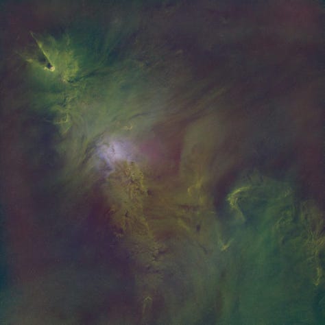
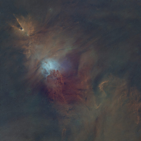
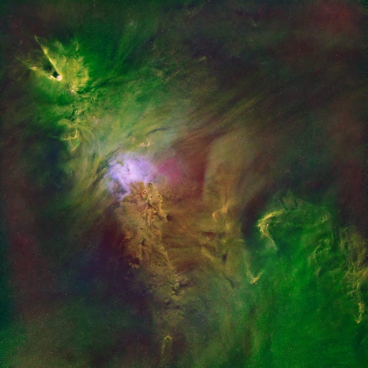
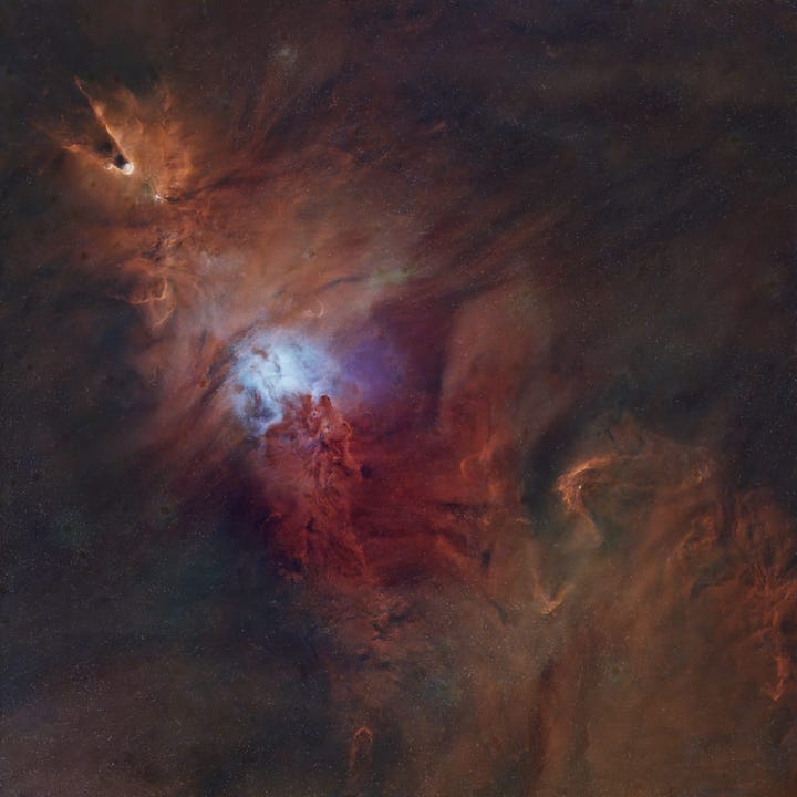
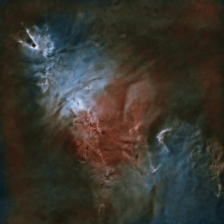
   I used PixelMath process, NBRGBCombinationx and SHO-AIP scripts to produce four image versions:

   • HOO

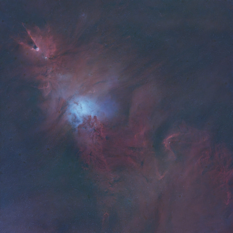
   • SHO (Hubble palette)

   • HHO

   • Foraxx (a weighted SHO variant)

   Before building the final palettes, I first tried to strengthen my OIII signal, because in my dataset OIII is the weakest channel (partly because I only managed one OIII night).

   To maximize it, by using PixelMath process I combined the two channels where OIII actually lives (green and blue) into a new single monochrome image, then creating OIII_base = 0.4 * OIII_G + 0.6 * OIII_B

   This isn’t magic: it’s simply a way to use both green and blue channels to squeeze the most out of the OIII frames.
   From there I generated four different versions. The idea wasn’t to prove one “correct” palette—there isn’t one—but to explore how different mappings emphasize different structures.

   • Classic HOO palette
     (Hα → Red, OIII → Green/Blue)
     
     This is one of the most common narrowband renderings: strong Hα provides the red structure, and OIII adds cyan/blue-green features.
     I used NBRGBCombination process with:

     • RGB Source Image: LPRO_starless, bandwidth 200nm.

     • Narrowband for R channel: LXT_R, 7nm, scale 1.20

     • Narrowband for G channel: OIII_G, 5nm, scale 1.50

     • Narrowband for B channel: OIII_B, 5nm, scale 1.50

   • SHO / Hubble palette
     (SII → Red, Hα → Green, OIII → Blue)
     
     This is the classic “Hubble palette” mapping. It’s famous because it produces strong separation between different chemical/physical regions, even though the final colors are a deliberate mapping choice.
     I built this version using SHO-AIP script, assigning::

     • Image SII: SII_R

     • Image HA: LXT_R

     • Image OIII: OIII_base

     Then I mixed the channels with these weights:

     • Red channel: 75% SII, 25% HA (I borrow some of Hα’s strength to keep the red channel from collapsing into noise and to improve contrast.)

     • Green channel: 100% HA

     • Blue channel: 150% OIII (OIII is weak in my dataset, so I pushed it.).

   • HHO palette
     (Hα → Red and Green, OIII → Blue)
     
     This one is essentially “Hα everywhere”, using red and green to exploit the strong hydrogen signal and build a very bright, detailed structure, with OIII providing color separation in the blue.
     Again with NBRGBCombination:

     • RGB Source Image: LPRO_starless, bandwidth 200nm.

     • Narrowband for R channel: LXT_R, 7nm, scale 1.20

     • Narrowband for G channel: LXT_G, 7nm, scale 1.20

     • Narrowband for B channel: OIII_G, 5nm, scale 1.50

   • Foraxx (a weighted SHO variant)
     This is a more “weighted” SHO-like rendering.
     
     I started by creating a balanced OIII mix with PixelMath, to generate a new monochrome image OIII_forax = (0.5 * OIII_G + 0.5 * OIII_B).
     Then I used ChannelCombination to build a basic SHO-style RGB:

     • R = SII_R

     • G = LXT_R

     • B = OIII_forax

     Finally, I applied PixelMath to slightly cross-feed the channels and rebalance the look:

     • R: 0.90*$T[0] + 0.10*$T[1]

     • G: 0.10*$T[1] + 0.90*$T[2]

     • B: 0.90*$T[2] + 0.10*$T[1]

     (Think of it as a controlled “mix” between adjacent channels to tame harsh separations and produce a smoother result.)

   

   Palette HHO, SHO, HHO (for some reason, I did not save the Foraxx base image)

9. Noise reduction
   Once the four palette versions were built, I applied NoiseXTerminator (NXT) process to each of them. At this stage I’m still in the starless domain, so noise reduction is easier to control without damaging star profiles.

10. Images histogram stretching
    This is a surprisingly delicate step for these images.

    Because each RGB channel in these composites comes from a different dataset (or a different extracted channel), the usual “natural correlation” between R/G/B histograms simply doesn’t exist. Many standard stretch tools can behave unpredictably in this situation.
    For that reason, the method that has been most reliable for me here is very simple: I apply an STF to get a visually balanced stretch, and then transfer that STF directly to HistogramTransformation (HT) process. It’s not the only possible approach, but in my experience it’s the least likely to produce weird channel relationships or color breakdowns with these mixed-source narrowband RGB images.

11. Local contrast + controlled color shaping
    After the stretch, I used LocalHistogramEqualization (LHE) process to enhance small-scale structure and microcontrast in the nebula. To avoid harsh effects, I applied LHE through a luminance-based mask (extracted from each image), so the contrast boost mostly targets nebular structure rather than amplifying background noise.
    LHE parameters (all four images):

    • Kernel radius: 64

    • Contrast limit: 2.0

    • Amount: 70%

    Then I used CurvesTransformation process for controlled contrast and saturation adjustments, trying to keep each palette’s identity while making it visually coherent and readable.
    At the end of the PixInsight workflow, I exported the four starless results as 16-bit TIFF.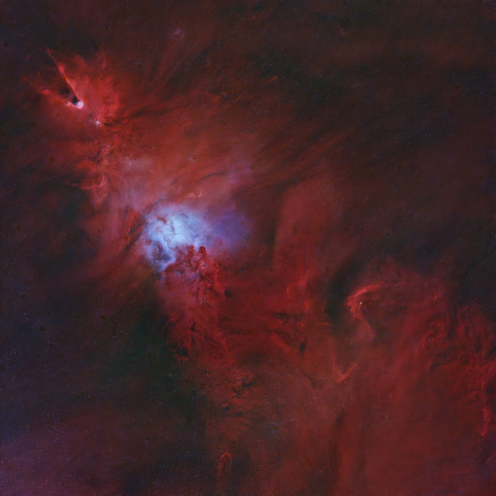

    

    

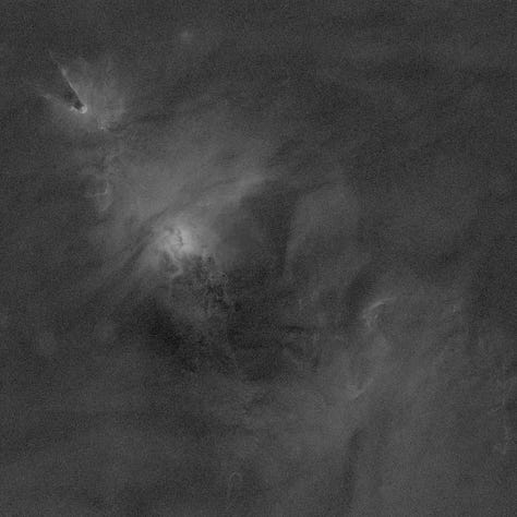
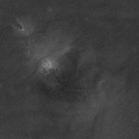
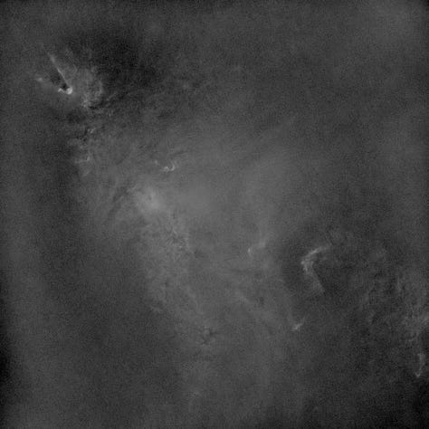
    From left to right, from top to bottom: HOO, SHO, HHO and Foraxx starless images, out of PixInsight workflow.

In parallel, I processed the star field extracted from LPRO_master.

I stretched LPRO_stars (again by transferring STF to HT), created a mask with StarMask process (default parameters), and used MorphologicalTransformation process three times (default settings) to gently reduce star sizes. Then I exported the star layer as a 16-bit TIFF.

At this point, it’s time to move to Photoshop.

Photoshop finishing + stars reintegration

Up to here the workflow is fairly structured—almost “scientific” in spirit—because it follows established narrowband processing logic.

Once you enter Photoshop, the truth is: the lab coat comes off. This is where we move from strict signal handling into creative interpretation, and the line between “processing” and “cheating” becomes a never-ending philosophical debate.

Personally, I use Photoshop to boost the colors, restore stronger contrast, correct local imperfections and adjust the overall color balance whenever it looks (to me) unsatisfying, and finally to add back the stars I previously extracted in PixInsight.

It’s fair to point out that all of these operations can also be done entirely within PixInsight, which is, after all, a platform specifically designed for astronomical image processing—and, in fact, the hardcore astrophotographers do exactly that. As for me, I strongly prefer Photoshop for these final steps, for a few very specific reasons:

• The ability to use precise, tightly localized masks to apply corrections only to very small and well-defined areas of the image. In that sense, working with masks in PixInsight can be a real nightmare—if not downright impossible, or at least it is with my current level of knowledge of the platform.

• A much more advanced and sophisticated color workflow, which allows you to intervene locally and very selectively. From this point of view, PixInsight’s CurvesTransformation process—which I do use for a first, rough refinement—feels primitive and frustratingly coarse compared to Photoshop.

• The countless possibilities offered by very flexible correction tools, such as the Clone Stamp. PixInsight does have similar tools, but compared to Photoshop it feels like prehistory.

• And finally—possibly the most important aspect—layer management. Every phase of my editing work in Photoshop relies on layers, especially the controlled way I reintroduce the stars on top of the nebula, which is entirely built around this mechanism.

So before reaching the final step—putting the stars back where they belong—I opened my four 16-bit TIFF images in Photoshop and placed them into a single PSD file, assigning each one to a separate layer. This allows me to work on all versions while quickly replicating the same adjustments across them, and above all it gives me an immediate, direct comparison: I can simply toggle layers on and off and see, instantly, how the different versions behave.

Not only that: I can also take advantage of layer opacity and blending options to experiment with further combinations, extracting the best characteristics from one version and injecting them into another. The possibilities are endless.

In this specific process, though, the goal is to stay true to the nature of each of the four versions and simply improve their appearance: make them brighter, apply small color balance adjustments, or tone down overly strong casts.

So I work on each image individually, making small color adjustments on its own layer, cleaning artifacts left from PixInsight using the Dust & Scratches filter, reducing noise a bit further in those sky areas where PixInsight’s algorithms didn’t manage to fully “smooth” the background, and boosting saturation where needed. Personally, I tend to like my images with fairly vivid, “lit up” colors—while still trying to preserve the original hues and their relationships as much as possible. That said, most truly skilled astrophotographers usually prefer images that are perhaps more muted, but definitely more restrained than mine—less “pop”, so to speak.

The key step, however, is the final overlay of the star layer. What is typically done in PixInsight via PixelMath becomes perfectly controllable in Photoshop: you place the stars layer above the nebula layers and choose the blending mode that defines how it interacts with what sits underneath.

My usual choice is “Screen” (Italian UI: Scolora): it removes the dark sky and brings out only the stars over the nebula without blowing out their brightness—keeping them intentionally subdued so they don’t steal the spotlight from the nebula.

Then I work directly on the stars layer itself: I completely eliminate residual shadows and further reduce highlights, with the goal of removing any leftover darkness that might veil the nebula beneath, and of weakening the stars’ saturation even more.

How prominent the stars should be in the final images is one of those topics that people can debate forever, and in the end it comes down to personal taste. Personally, I prefer the viewer’s attention to be captured by the nebula’s structure and detail, rather than by a dense, bright carpet of stars that competes with it and ends up covering too much of its character.

Final images are at the top. If you’re into this kind of thing, I’m happy to go deeper on any step (or on why I keep choosing pain). Questions, comments, and constructive nitpicking are welcome.

And that’s all. Clear sky!